Route compactness

Route compactness refers to the geographic density of nodes (customers) in a single route. Compact routes keep stops close together, minimizing travel and giving each vehicle a focused service territory.

The solver exposes two mechanisms to encourage compactness, usable independently or together:

• Spatial dispersion penalty (cluster_cost) — penalizes how spread out each vehicle's nodes are around their centroid. Operates directly on node coordinates.
• Travel-cost shaping (travel_matrix_operator / route_cost_modification_*) — penalizes long or expensive travel legs. Operates on the time/distance matrices.

Impact on planning

Efficiency: Compact routes reduce stem time (depot to service area) and route time (between customers).

Driver familiarity: Drivers get to know their own zones — faster service, fewer wrong turns, and easier handoffs between shifts.

Customer service: Tighter service areas support more reliable delivery windows and faster response.

Scalability: New customers slot into the nearest existing cluster; new vehicles open new clusters.

Example

A catering company has 100 orders across a city and 5 vans (20 orders each).

• Without compactness: routes zigzag and overlap. One van crosses the city north-to-south while another does the reverse.
• With compactness: each van owns one cluster — Downtown, West Suburbs, etc. Stops for any single van stay in one neighborhood, cutting travel time and operational cost.

Cluster cost penalty

cluster_cost penalizes how spread out each vehicle's nodes are around their geometric center, pushing the solver toward compact, non-overlapping territories. It operates on node

coordinates directly — useful when travel-cost shaping alone fails to break ties between dispersed and tight routes that look similar in travel time.

How it works

For each vehicle, the solver finds the geographic centre of all its assigned stops, then measures how far each stop sits from that centre. The further apart the stops are from one another, the larger the penalty added to the route cost — so the solver naturally prefers solutions where each vehicle's stops cluster tightly together. The factor parameter controls how strongly this penalty competes with the usual travel-time and distance costs.

Effect of factor

Disabled by default — both use_cluster_radius: true and factor > 0 are required to activate.

factor	Behavior
0	Disabled. Pure time/distance optimization.
5–10	Mild bias. Small travel impact.
10–20	Visibly tight clusters. Recommended starting range.
> 20	Aggressive. Solver accepts noticeably longer travel for tighter clusters.

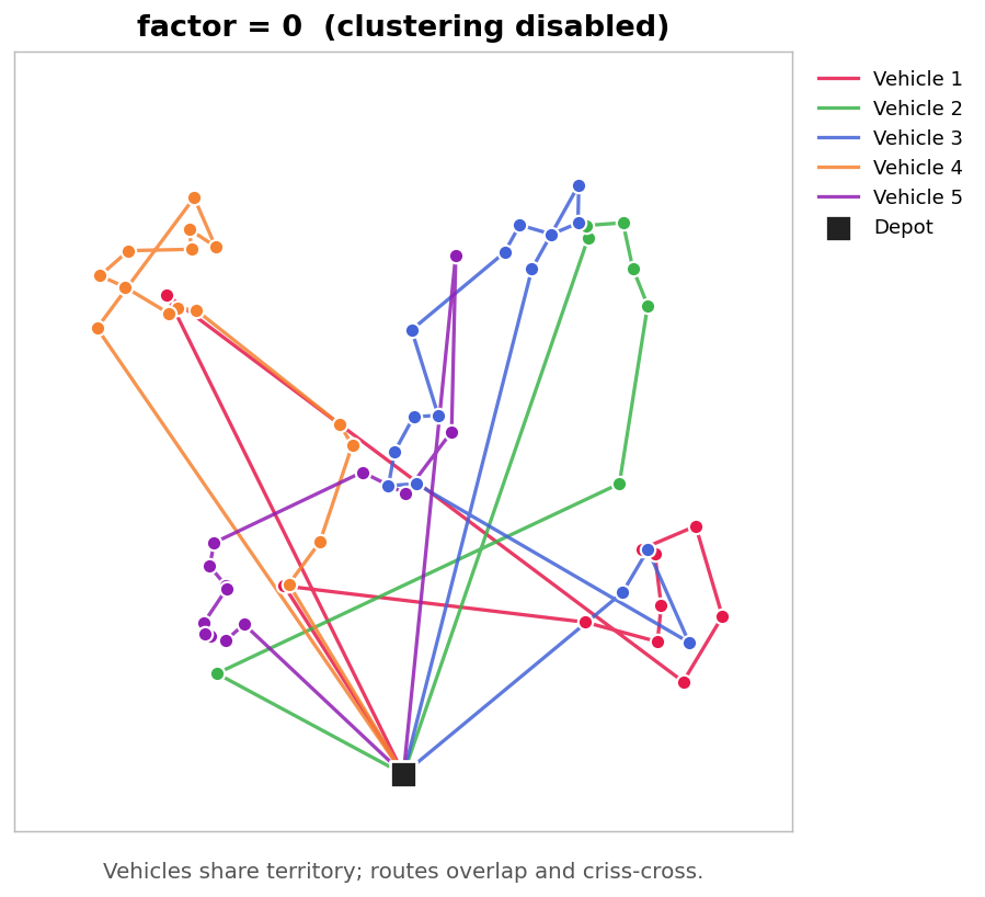
factor = 0 — clustering disabled. Vehicles share territory and routes criss-cross.

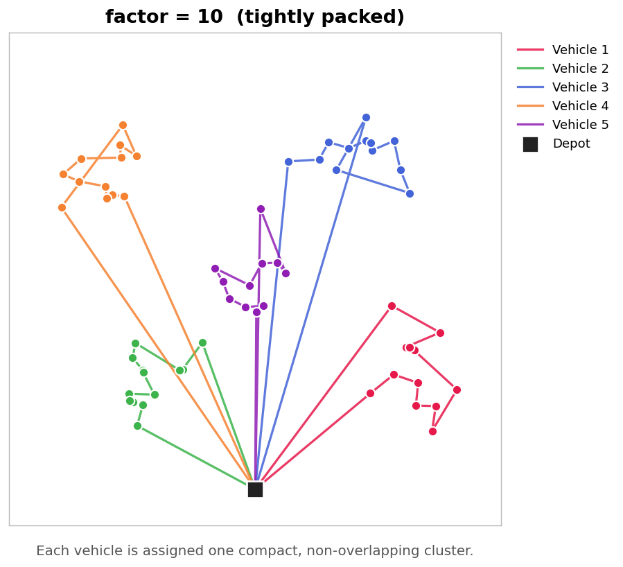
factor = 10 — each vehicle owns a compact, non-overlapping territory.

Configuration (Integration API)

Configure under simulation.data.logistics_api_settings.cluster_cost. Set to null (or omit) to disable.

PATCH /api/v2/simulation/{id}

{
    "data": {
        "logistics_api_settings": {
            "cluster_cost": {
                "use_cluster_radius": true,
                "factor": 10
            }
        }
    }
}

Parameters

Parameter	Type	Default	Description
use_cluster_radius	boolean	false	Master switch. Must be true to enable.
factor	integer	0	Clustering strength. Must be > 0. Squared internally.
ignore_node_types	list of string	["depot", "vehicle_position"]	Node types excluded from clustering. Replaces the default — re-include "depot" and "vehicle_position" if you extend the list.
ignore_latlons	list of [lat, lon]	[]	Specific coordinates to exclude (e.g. a shared transfer point that would otherwise skew centroids).

Example: exclude a shared transfer point

PATCH /api/v2/simulation/{id}

{
    "data": {
        "logistics_api_settings": {
            "cluster_cost": {
                "use_cluster_radius": true,
                "factor": 12,
                "ignore_latlons": [[1.290270, 103.851959]]
            }
        }
    }
}

Biases the solver toward compact territories (factor: 12) while keeping a known shared point out of the centroid math, so it doesn't pull every vehicle's centre toward itself.

Starting point

Start at factor: 10. Double if clusters still look loose, halve if travel time degrades noticeably. Above 20 is aggressive.

ignore_node_types replaces, not appends

Re-include "depot" and "vehicle_position" whenever you extend the list.

Travel-cost shaping (travel_matrix_operator)

travel_matrix_operator replaces the standard route-cost calculation with a configurable expression over the time and distance matrices, letting you apply linear and step-function penalties to individual travel legs. Available in engine_settings.model_parameters (Stateless API).

The total route-dependent cost sums contributions from the primary and secondary routing engines:

$${\tt cost} = R(\widetilde{T}_{ij}^{(1)})+R(\widetilde{D}_{ij}^{(1)})+R(\widetilde{T}_{ij}^{(2)})+R(\widetilde{D}_{ij}^{(2)})$$

Superscripts (1) and (2) refer to the primary and secondary engines. $\widetilde{T}_{ij}$ and $\widetilde{D}_{ij}$ are the time and distance matrices. Each $R()$ combines a linear term and any number of polylinear penalties:

$$R({m}_{ij}) = m_{ij} \cdot {\tt linear} + \sum_k[({\tt base}_k + (m_{ij}-{\tt threshold}_k) \cdot{\tt rate}_k), \; {\tt if} \;m_{ij}>{\tt threshold}_k]$$

Each polylinear rule $k$ applies its penalty when $m_{ij}$ crosses threshold.

Configuration (Stateless API)

engine_settings.model_parameters.travel_matrix_operator

{
    "travel_matrix_operator": {
        "use_optimize_quantity": false,
        "primary": {
            "time": {
                "linear": 1,
                "polylinear": [
                    {
                        "threshold": 3600,
                        "relation": "greater",
                        "penalty": { "base": 5000, "rate": 2 }
                    }
                ]
            },
            "distance": { "linear": 0.5 }
        },
        "secondary": {
            "distance": {
                "linear": 0.1,
                "polylinear": [
                    {
                        "threshold": 10000,
                        "relation": "greater",
                        "penalty": { "base": 1000, "rate": 0.2 }
                    }
                ]
            }
        }
    }
}

Key parameters

• use_optimize_quantity (boolean, default false):

  • true: backward-compatible mode — only the matrix matching optimize_quantity contributes. If optimize_quantity = "total_distance", primary.time and secondary.time are ignored.
  • false: optimize_quantity is ignored and every parameter in travel_matrix_operator contributes.

• primary and secondary: cost contributions from two independent routing engines. A common pattern is primary = osrm (real road network) and secondary = spheroid (straight-line). A small linear factor on the secondary distance penalizes geographic dispersion without overriding the primary objective.

• Within each engine, time and distance accept:

  • linear (number, default 0): scaling factor on $m_{ij}$. 1 adds the travel value as-is; 2 doubles it.
  • polylinear (array): step-function penalty rules — see below.

polylinear rules

Each entry in polylinear:

• threshold (number, default 0): trigger value. Units match the matrix (seconds for time, meters for distance).
• relation (string, required): "greater" or "less".
• penalty (object, default {"base": 0, "rate": 0}):
  • base: fixed penalty when the condition is met.
  • rate: additional penalty per unit beyond the threshold.
• ignore_first (default true): skip the trip from partial_route (depot) to the first stop.
• ignore_last (default true): skip the trip from the last stop back to partial_route_end.

Notes

• For relation: "less", rate must be negative to yield a positive penalty.
• Multiple polylinear rules sum independently.
• Total leg cost is clamped to non-negative values.
• Mixed fleets can differ via matrix_id.

Practical example

Goal: minimize travel time, penalize trips over 1 hour, encourage geographic compactness.

engine_settings

{
    "routing_engine": { "routing_engine_name": "osrm" },
    "secondary_routing_engine": { "routing_engine_name": "spheroid" },
    "model_parameters": {
        "travel_matrix_operator": {
            "use_optimize_quantity": false,
            "primary": {
                "time": {
                    "linear": 1,
                    "polylinear": [
                        {
                            "threshold": 3600,
                            "relation": "greater",
                            "penalty": { "base": 5000, "rate": 2 }
                        }
                    ]
                }
            },
            "secondary": {
                "distance": { "linear": 0.1 }
            }
        }
    }
}

• primary.time.linear: 1 makes total travel time the main cost.
• primary.time.polylinear: trips over 3600s incur a base: 5000 penalty plus rate: 2 per second over.
• secondary.distance.linear: 0.1: a small straight-line penalty breaks ties toward closer stops, promoting compactness.

Configuration (Integration API)

Integration API exposes the same mechanism via two simulation.data.logistics_api_settings fields that mirror the primary and secondary blocks:

• route_cost_modification_primary — primary routing engine.
• route_cost_modification_secondary — secondary routing engine.

Each accepts an object with time and distance keys using the linear / polylinear structure above.

PATCH /api/v2/simulation/{id}

{
    "data": {
        "logistics_api_settings": {
            "route_cost_modification_primary": {
                "time": {
                    "linear": 1,
                    "polylinear": [
                        {
                            "threshold": 3600,
                            "relation": "greater",
                            "penalty": { "base": 5000, "rate": 2 }
                        }
                    ]
                }
            },
            "route_cost_modification_secondary": {
                "distance": { "linear": 0.1 }
            }
        }
    }
}

Equivalent to the stateless practical example above.

Parameter	Type	Description
route_cost_modification_primary	object	Cost modification for the primary routing engine. Accepts time and distance keys.
route_cost_modification_secondary	object	Cost modification for the secondary routing engine. Accepts time and distance keys.

See Logistics API Settings for the full list.

Pair the two mechanisms carefully

cluster_cost and travel_matrix_operator push toward shorter / tighter routes via different signals. Enabling both at high weight can over-constrain the solver and increase booking rejections — tune them one at a time.

Playground

Try the Route Compactness concept with the playground below.

Loading...