On demand routing and operations

On-demand operations in the Vehicle Routing Problem (VRP) refer to scenarios where customer requests (orders) are not known in advance but rather arise dynamically in real-time. This contrasts with traditional VRP models where all orders are typically assumed to be known beforehand.

tip

While this use case centers around passenger travel, which is the most typical use case for on-demand services, it is also applicable to live order management in other industries, such as logistics.

Key Characteristics of On-Demand VRP:

• Dynamic Requests: Customers place orders with varying delivery locations and requirements throughout the operational period.
• Real-time Decision Making: The system must react to new incoming orders and adjust vehicle routes dynamically.
• Uncertainty: The future demand is unknown, making planning and optimization more complex.

On-demand operations significantly increase the complexity of the VRP solution compared to static VRPs.

• Continuous Re-optimization: As new orders arrive, the existing routes need to be re-optimized to incorporate the new requests efficiently. This requires frequent re-planning and can be computationally intensive.
• Real-time Response: The system needs to respond quickly to new orders to provide timely service to customers. This necessitates efficient algorithms and potentially real-time communication with vehicles.
• Uncertainty Management: Dealing with unknown future demand requires incorporating uncertainty into the planning process. This might involve using probabilistic models or robust optimization techniques to account for potential variations in demand.
• Dynamic Constraints: Time windows and other constraints might also be dynamic, changing as new orders come in. This adds another layer of complexity to the optimization problem.

Challenges and Considerations:

• Algorithm Efficiency: Algorithms for on-demand VRP need to be efficient enough to handle real-time updates and re-optimization.
• Information Management: The system needs to effectively manage information about incoming orders, vehicle locations, and changing constraints.
• Communication: Real-time communication between the central system and the vehicles is crucial for dynamic routing.
• Customer Service: Balancing efficiency with customer service is essential. The system needs to provide reasonable delivery time estimates and manage customer expectations in the face of dynamic changes.

Examples of On-Demand VRP:

• Courier Services: Companies like FedEx or UPS deal with on-demand requests for package pickups and deliveries.
• Ride-Sharing Services: Uber and Lyft operate on a purely on-demand basis, matching riders with available drivers in real-time.
• Food Delivery Services: Services like DoorDash or Grubhub handle orders that come in dynamically from customers.

SWAT APIs support operations on-demand, making such workflows applicable to both logistics and people transport scenarios.

Service quality parameters

Quality of on demand services can be configured to support various types of operations, including:

• "Taxi" model riding (one trip per vehicle)
• On demand pooling
• Support for walking for the passengers for a pickup at a predefined location

The quality of service is determined by the passengers' waiting time, trip duration, and cost of the trip.

SWAT model supports the following cost function with the objective of it's minimization:

• Optimization goals:
  • Optimize total time (cost function is set in seconds and respects all configured time-based parameters)
  • Optimize total distance (cost function is set in meters and respects all configured distance-based parameters)
  • Passenger optimization (removes all vehicle related costs)
• Vehicle related costs:
  • Vehicle trips (sum of duration of all vehicle trips)
  • Vehicle cost (cost of using the vehicle)
• Passenger related costs:
  • Passenger trips (sum of durations of all passenger trips)
  • Passenger walking (additional cost allowing passengers to walk to\from the pickup\drop off location)
• Penalties:
  • Some constraints can be soft, there is penalty for breaking them

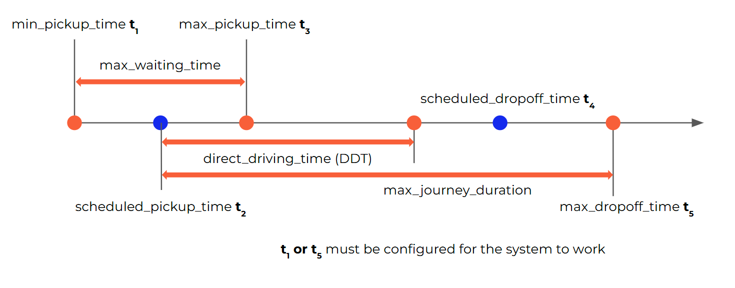
On of the key parameters for service quality is maximum waiting time for a passenger for a pickup. This time window is controlled by acceptable_waiting_time parameter.

Another parameter that controls the ability to pool passengers and determines service quality is the maximum journey duration for a passenger. Several methods are supported to calculate the cost related to journey duration, including:

Value	Maximum journey duration
constant	max_additional_journey_time
routing	DDT + max(max_additional_journey_time, DDT * max_additional_journey_time_percent)
routing_max_cap	min(absolute_max_trip_duration, DDT + max(max_additional_journey_time, DDT * max_additional_journey_time_percent)
routing_min	DDT + min(max_additional_journey_time, DDT * max_additional_journey_time_percent)
routing_min_cap	min(absolute_max_trip_duration, DDT + min(max_additional_journey_time, DDT * max_additional_journey_time_percent)
different	max_dropoff_time - min_pickup_time

The calculation mode is controlled by the simulation.journey_duration_source parameter.

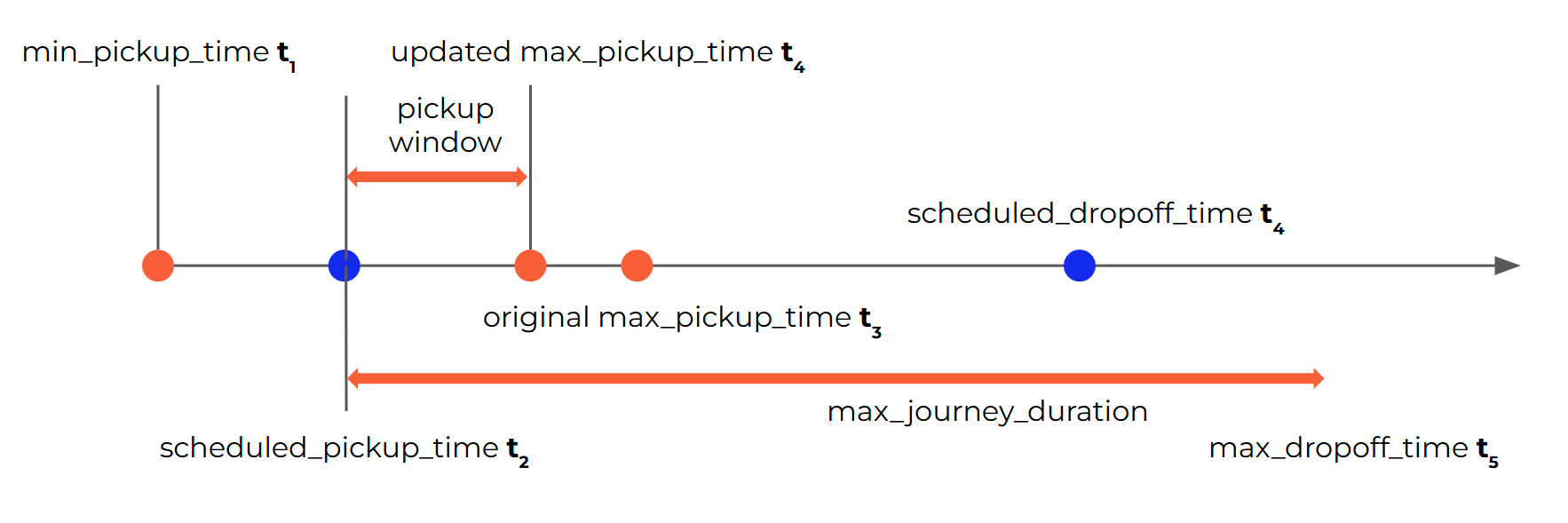
Insertion of a new booking

New bookings can be added to the same vehicle only if the constraints (pickup and dropoff windows) are not violated for the new and existing bookings on that vehicle. For successful insertion, any time window or other types of constraints must be met. Supporting flexible time windows allow for adjusting initial plan for the vehicle(s) without breaking the constraints.

Walking to the locations

The SWAT algorithm supports the ability for passengers to walk to a specific predefined stop as part of the optimization process. If there are mulitple pickup locations available in the proximity, then the best one (based on selected optimization criteria) will be offered.

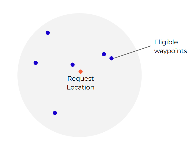
For requested pickup location A, if max walking distance is > 0, the system will finds the waypoints in the indicated transitstopset within that walking Distance range.

These waypoints will be possible pickup locations for the booking. The algorithm will decide which one is more suitable for the pickup.

Walking time or distance can be included in the cost function to show a preference for closer stops.

Example:

System configuration:

• simulation.data.max_distance_to_neighbor_stops = 300
• simulation.data.max_number_of_neighbor_stops = 4
• simulation.data.calculation_parameters.node_weight_coeff = 0.5

Result:

• Find all the waypoints within 300m from the requested location
• If more than 4, only take the closest 4 waypoints
• The 4 waypoints will be the pickup nodes for the booking
• For any node selected, the overall cost function + 0.5 * walking_time